Since heavy-ion collisions produce a very high multiplicity of particles, a statistical treatment of the system can be adopted. If thermal equilibrium is reached, the system is characterized by thermodynamic observables, such as volume, lifetime, temperature and energy density.
The expected space-time evolution of a heavy-ion collision - with and without QGP formation - is shown in fig. 1.4.
|
Identical-particle interferometry, also referred to as Hanbury-Brown-Twiss
(HBT) correlations [8], e.g. ![]() or KK correlations,
can be used to study the space-time dynamics of nuclear collisions.
From such two-particle correlations it is possible to obtain
information on the transverse and longitudinal size, on the lifetime and
on flow patterns of the source at the freeze-out time. For instance,
different particle species may freeze out at different times and give
different source sizes, due to the expansion of the source.
or KK correlations,
can be used to study the space-time dynamics of nuclear collisions.
From such two-particle correlations it is possible to obtain
information on the transverse and longitudinal size, on the lifetime and
on flow patterns of the source at the freeze-out time. For instance,
different particle species may freeze out at different times and give
different source sizes, due to the expansion of the source.
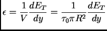
With a hydrodynamic description of the colliding system, the energy density ![]() can be estimated for central collisions from the transverse energy per unit rapidity as
can be estimated for central collisions from the transverse energy per unit rapidity as
Here ![]() is the radius of the participant zone
and
is the radius of the participant zone
and ![]() is the proper formation time. Usually a value of
is the proper formation time. Usually a value of
![]() = 1 fm/c is used.
= 1 fm/c is used.
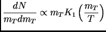
The particle emission from a source in thermal equilibrium is Maxwell-Boltzmann distributed according to [9]
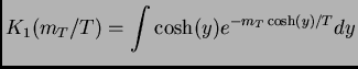
where ![]() is the modified Bessel function
is the modified Bessel function
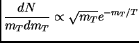
With the assumption that ![]() eq. 1.10 can be approximated as
eq. 1.10 can be approximated as
The temperature would then be given by the inverse slope of a semilogarithmic
plot of
![]() vs.
vs. ![]() .
.