Influences on the Fluctuations

Since charge is a globally conserved quantity, the fluctuation measurements are strongly dependent on the acceptance of the detector. If all charged particles, denoted $N_{ch}$, are detected in each event, i.e. with 100% detection efficiency and a $4\pi$ detector, there are no fluctuations, and $v(Q)=0$.

Another property that may alter the magnitude of the fluctuations is charge asymmetry, i.e. when - for some reason - more positive than negative particles are detected or vice versa. This was seen already in (3.1). With $\varepsilon \equiv p_+-p_-$ representing a small excess of positive particles, $v(Q)=4p_+p_-=1-\varepsilon^2$ in this case.

Neutral resonances, such as $\rho$ and $\omega$, introduce positive correlations between $n_+$ and $n_-$ and therefore reduce the fluctuations. In [17] Jeon and Koch estimate the reduction to $v(Q)=0.75$.This effect will be examined in simulations in section 3.2.

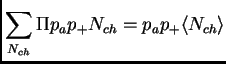
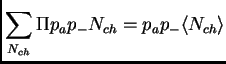
Global charge conservation and charge asymmetry can be incorporated into one calculation to yield a more general result for $v(Q)$. Let $p_a$ denote the fraction of observed charged particles among all charged particles in the event. In the following derivation both $n_{ch}$ and $n_+(n_-)$ are binomially distributed (with probabilities $p_a$ and $p_+(p_-)$, and the probability distribution for $N_{ch}$ is denoted $\Pi$. It is also assumed that the ratio between $N_+$ and $N_-$ is constant. First, a few building blocks needed to find the expression for V$(Q)$:

$$\<n_+\> = \sum_{N_{ch}} \Pi p_a p_+ N_{ch} = p_a p_+ \<N_{ch}\>$$ (19)

$$\<n_-\> = \sum_{N_{ch}} \Pi p_a p_- N_{ch} = p_a p_- \<N_{ch}\>$$ (20)

$$\<n_+^2\> = \sum_{N_{ch}} \Pi \left[p_a(1-p_a)p_+N_{ch} + p_a^2p_+^2N_{ch}^2\right] =$$

$$= p_a(1-p_a)p_+\<N_{ch}\> + p_a^2p_+^2\<N_{ch}^2\>$$ (21)

$$\<n_-^2\> = \sum_{N_{ch}} \Pi \left[p_a(1-p_a)p_-N_{ch} + p_a^2p_-^2N_{ch}^2\right] =$$

$$= p_a(1-p_a)p_-\<N_{ch}\> + p_a^2p_-^2\<N_{ch}^2\>$$ (22)

$$\<n_+n_-\> = \sum_{N_{ch}} \Pi p_a^2p_+p_-N_{ch}^2 = p_a^2p_+p_-\<N_{ch}^2\>$$ (23)

Using equations (3.7) - (3.11) the expression for V$(Q)$ is

$$\mt{V}(Q) \equiv \<Q^2\>-\<Q\>^2 = \<(n_+-n_-)^2\> - \<n_+-n_-\>^2 =$$

$$= \<n_+^2\> + \<n_-^2\> - 2\<n_+n_-\> - \<n_+\>^2 - \<n_-\>^2 + 2\<n_+\>\<n_-\> =$$

$$= p_a(1-p_a)p_+\<N_{ch}\> + p_a^2p_+^2\<N_{ch}^2\> + p_a(1-p_a)p_-\<N_{ch}\> +p_a^2p_-^2\<N_{ch}^2\> -$$

$$- 2p_a^2p_+p_-\<N_{ch}^2\> - p_a^2p_+^2\<N_{ch}\>^2 - p_a^2p_-^2\<N_{ch}\>^2 + 2p_a^2p_+p_-\<N_{ch}\>^2 =$$

$$= p_a(1-p_a)\<N_{ch}\> + p_a^2(p_+^2+p_-^2-2p_+p_-)\<N_{ch}^2\> -$$

$$- p_a^2(p_+^2+p_-^2-2p_+p_-)\<N_{ch}\>^2 =$$

$$= (1-p_a)\<n_{ch}\> + p_a^2\varepsilon^2\mt{V}(N_{ch})$$ (24)

V$(n_{ch})$ can be used in order to express V$(N_{ch})$ in terms of $n_{ch}$:

$$\mt{V}(n_{ch}) \equiv \<n_{ch}^2\> - \<n_{ch}\>^2 =$$

$$= \sum_{N_{ch}} \Pi \left[p_a(1-p_a)N_{ch} + p_a^2N_{ch}^2\right] - p_a^2\<N_{ch}\>^2 =$$

$$= p_a(1-p_a)\<N_{ch}\> + p_a^2\<N_{ch}^2\> - p_a^2\<N_{ch}\>^2 =$$

$$= p_a(1-p_a)\<N_{ch}\> + p_a^2\mt{V}(N_{ch})$$ (25)

Using (3.13) in (3.12) yields

$$\mt{V}(Q) = (1-p_a)\<n_{ch}\> + \varepsilon^2 \cdot (\mt{V}(n_{ch})-(1-p_a)\<n_{ch}\>) =$$

$$= (1-p_a)(1-\varepsilon^2)\<n_{ch}\> + \varepsilon^2\mt{V}(n_{ch})$$ (26)

and the result can finally be given with normalized variances:

$$v(Q) = (1-p_a)(1-\varepsilon^2) + \varepsilon^2v(n_{ch})$$ (27)

Experimental effects, such as background contributions and detection inefficiencies, also influence the magnitude of the fluctuations. The effect of a background consisting of uncorrelated positive and negative particles can easily be estimated. The observed variance V$_{obs}(Q)$ is the sum of the true and background contributions.

$$\mt{V}_{obs}(Q) = \mt{V}_{true}(Q) + \mt{V}_{bkg}(Q)$$ (28)

With $f_{bkg}$ being the fraction of the particles coming from background,

$$v_{obs}(Q) = (1-f_{bkg}) \cdot v_{true}(Q) + f_{bkg} =$$

$$= 1 - (1-f_{bkg}) (1-v_{true}(Q))$$ (29)

Background contributions move a reduced $v(Q)$ towards the value 1, the stochastic scenario. Detection inefficiencies affect the fluctuations in a similar way. Assuming that the detection efficiency $p_e$ is equal for positive and negative particles,

$$v_{obs}(Q) = 1 - p_e (1-v_{true}(Q))$$ (30)

The combined result can be obtained by substituting $v_{obs}(Q)$ of (3.18) into $v_{true}(Q)$ in (3.17):

$$v_{obs}(Q) = 1 - p_e (1-f_{bkg}) (1-v_{true}(Q))$$ (31)